LabPlot/ComputationalNotebooks: Difference between revisions
No edit summary |
add about CAS Computing |
||
| Line 10: | Line 10: | ||
{{#ev:youtube|8lDQStVDevw|800|center}} | {{#ev:youtube|8lDQStVDevw|800|center}} | ||
<nowiki> | |||
With this, powerful calculations carried out inside of different CAS environments can be combined with the user-friendly visualisation and editing capabilities of LabPlot. This combination is demonstrated below with the help of two examples: | |||
</nowiki> | |||
[[File:Labplot2 appdata 03.png|frameless|center|upright=3.0]] | |||
<center> | |||
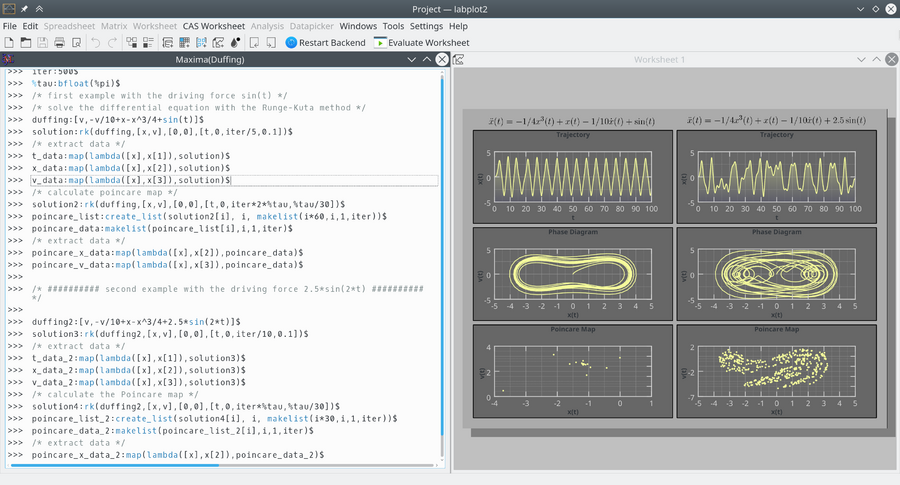
Maxima session showing the chaotic dynamics of the Duffing oscillator. The differential equation of the forced oscillator is solved with Maxima. Plots of the trajectory, the phase space of the oscillator, and the corresponding Poincaré map are done with LabPlot. | |||
</center> | |||
[[File:Python session.png|frameless|center|upright=3.0]] | |||
<center> | |||
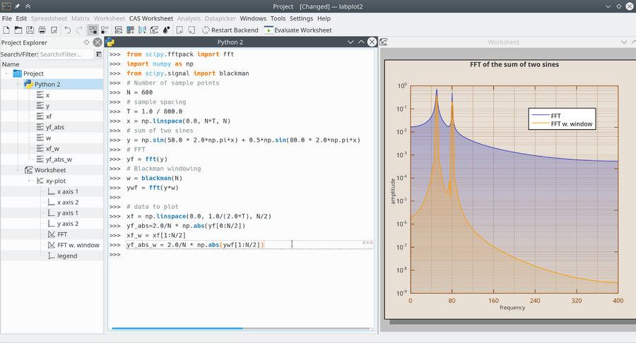
Python session illustrating the effect of Blackman windowing on the Fourier transform | |||
</center> | |||
Revision as of 02:01, 24 January 2024
LabPlot can be used as a frontend to different open-source computer algebra systems (CAS) like Maxima, Octave, R, Scilab, and Sage or programming languages providing similar capabilities like Python and Julia. LabPlot recognizes different CAS variables holding array-like data and allows selecting them as a source for curves. So, instead of providing columns of a spreadsheet as the source for x- and y-data, the user provides the names of the corresponding CAS-variables. Currently supported CAS data containers are
- Maxima lists
- Python lists, tuples and NumPy arrays
- Julia vectors and tuples
With this, powerful calculations carried out inside of different CAS environments can be combined with the user-friendly visualization and editing capabilities of LabPlot.
See the video on how to use Computational Notebooks in LabPlot.
{{#ev:youtube|8lDQStVDevw|800|center}}
With this, powerful calculations carried out inside of different CAS environments can be combined with the user-friendly visualisation and editing capabilities of LabPlot. This combination is demonstrated below with the help of two examples:

Maxima session showing the chaotic dynamics of the Duffing oscillator. The differential equation of the forced oscillator is solved with Maxima. Plots of the trajectory, the phase space of the oscillator, and the corresponding Poincaré map are done with LabPlot.

Python session illustrating the effect of Blackman windowing on the Fourier transform
